Data & Analytics Projects
Analytics engineering, machine learning and statistical analysis — from raw data to clean models and actionable insight.
 100k+ orders · Analytics Engineering
E-Commerce Data Platform — Olist Brazil
End-to-end data pipeline over 100k+ real orders from the Brazilian market (Olist). PostgreSQL + dbt with 4 model layers: staging → intermediate → marts. RFM segmentation, cohort retention, revenue trends and seller performance — all in pure SQL. Analysis and documentation written in Portuguese (C1). CI/CD with GitHub Actions.
-- mart_rfm_segmentation.sql (dbt model)
WITH rfm_base AS (
SELECT
customer_unique_id,
DATEDIFF('day', MAX(order_purchase_timestamp),
CURRENT_DATE) AS recency,
COUNT(DISTINCT order_id) AS frequency,
SUM(payment_value) AS monetary
FROM {{ ref('int_orders_enriched') }}
WHERE order_status = 'delivered'
GROUP BY 1
),
rfm_scores AS (
SELECT *,
NTILE(5) OVER (ORDER BY recency DESC) AS r_score,
NTILE(5) OVER (ORDER BY frequency) AS f_score,
NTILE(5) OVER (ORDER BY monetary) AS m_score
FROM rfm_base
)
SELECT *,
CASE
WHEN r_score >= 4 AND f_score >= 4 THEN 'Champions'
WHEN r_score >= 3 AND f_score >= 3 THEN 'Loyal'
WHEN r_score >= 4 AND f_score <= 2 THEN 'New Customers'
WHEN r_score <= 2 AND f_score >= 3 THEN 'At Risk'
ELSE 'Hibernating'
END AS segment
FROM rfm_scores 6,500+ measurements · Privacy-first
Athlete Performance Monitor — Demo Dataset
Synthetic dataset of 6,500+ CMJ/IMTP measurements generated in Python. Faker + numpy with distributions calibrated against sport-science literature. Neuromuscular alert system with dynamic p25/p75 thresholds and a 5-evaluation moving average. IDs hashed at the source — zero real personal data.
# Distribuciones calibradas con normas publicadas
SPORTS = {
"Fútbol": {"cmj": (42, 6), "imtp": (1_800, 300)},
"Rugby": {"cmj": (45, 7), "imtp": (2_200, 350)},
"Atletismo": {"cmj": (50, 8), "imtp": (2_000, 300)},
"Basketball": {"cmj": (55, 8), "imtp": (1_900, 300)},
}
def hash_id(raw: str) -> str:
return "ATH" + hashlib.sha256(raw.encode()).hexdigest()[:6].upper()
# Faker genera nombre → se hashea → nombre descartado
raw_name = fake.name()
athlete_id = hash_id(raw_name + sport) # único, anónimo
# Fatiga modelada como ruido multiplicativo ±7%
fatigue = float(rng.normal(1.0, 0.07))
jump_h = max(15.0, base_cmj * fatigue + rng.normal(0, 1.5))
max_force = max(500.0, base_imtp * fatigue + rng.normal(0, 30))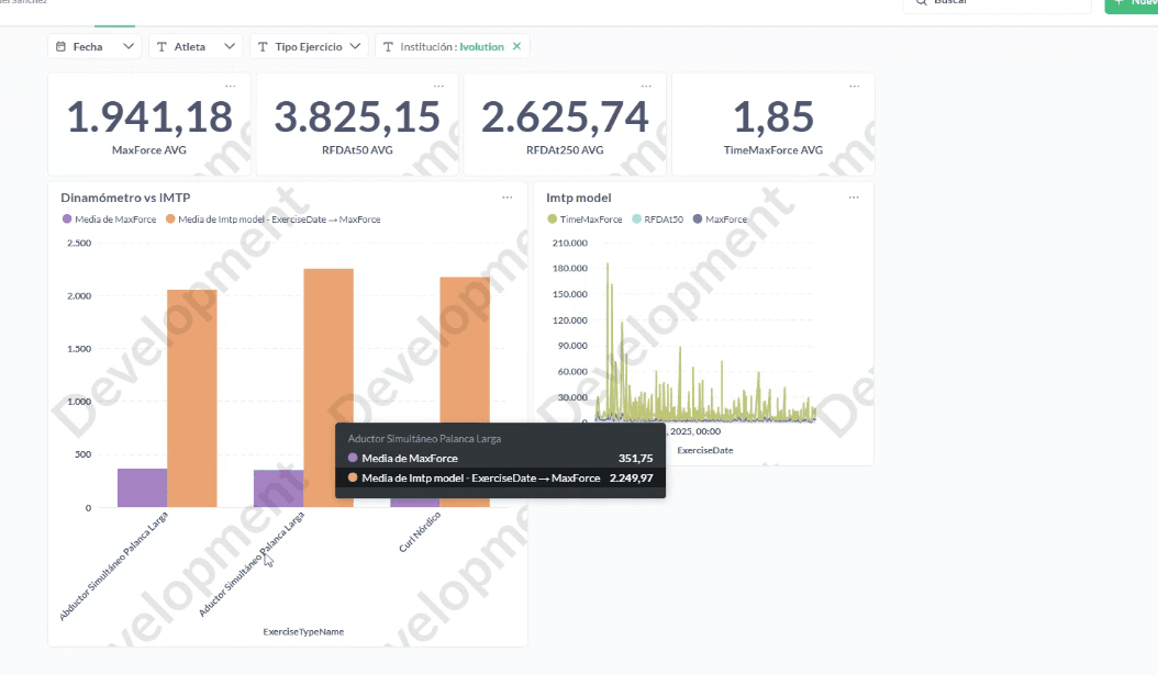 967 athletes · 13 sports
Performance Monitoring System — Ivolution
967 athletes monitored across 13 sports. Three-state alerts (SUPERCOMPENSATION / ATTENTION / FATIGUED) with dynamic percentile thresholds (p25/p75), 10,000+ recorded measurements and multilingual ES/EN/PT support. The system is still running after I left — the organization's main decision-making tool.
-- athlete_fatigue_alerts.sql (BigQuery + dbt)
WITH athlete_baseline AS (
SELECT
athlete_id,
exercise_type,
PERCENTILE_CONT(max_force, 0.25)
OVER (PARTITION BY athlete_id, exercise_type) AS p25,
PERCENTILE_CONT(max_force, 0.75)
OVER (PARTITION BY athlete_id, exercise_type) AS p75
FROM {{ ref('stg_measurements') }}
WHERE eval_date >= DATE_SUB(CURRENT_DATE(), INTERVAL 90 DAY)
),
latest_eval AS (
SELECT DISTINCT ON (athlete_id, exercise_type)
athlete_id, exercise_type, max_force, eval_date
FROM {{ ref('stg_measurements') }}
ORDER BY athlete_id, exercise_type, eval_date DESC
)
SELECT
l.athlete_id,
l.exercise_type,
l.max_force,
b.p25, b.p75,
CASE
WHEN l.max_force >= b.p75 THEN 'SUPERCOMPENSACIÓN'
WHEN l.max_force <= b.p25 THEN 'FATIGADO'
ELSE 'ATENCIÓN'
END AS estado
FROM latest_eval l
JOIN athlete_baseline b USING (athlete_id, exercise_type) 212,292 users · 6 segments
User Segmentation — Email Marketing
Unsupervised segmentation over 212,292 real records from mailing campaigns. Applies K-Means and MiniBatchKMeans with Silhouette Score analysis to find the optimal k (6 segments). PCA dimensionality reduction for visualization. Output: an Excel file with cluster assignments and tailored strategy recommendations per segment.
from sklearn.cluster import MiniBatchKMeans
from sklearn.preprocessing import StandardScaler
from sklearn.metrics import silhouette_score
import pandas as pd
scaler = StandardScaler()
X_scaled = scaler.fit_transform(df[features])
# Silhouette analysis to find optimal k
scores = {}
for k in range(2, 11):
model = MiniBatchKMeans(n_clusters=k, random_state=42)
labels = model.fit_predict(X_scaled)
scores[k] = silhouette_score(X_scaled, labels, sample_size=5000)
optimal_k = max(scores, key=scores.get) # k=6
final_model = MiniBatchKMeans(n_clusters=optimal_k, random_state=42)
df['cluster'] = final_model.fit_predict(X_scaled)
# Cluster profiling
profile = df.groupby('cluster')[features].mean()
profile['size'] = df['cluster'].value_counts() 1,470 employees
IBM HR Analytics — Attrition Prediction
End-to-end analysis of IBM's official dataset of 1,470 employees. Identifies the factors with the biggest impact on employee attrition using Random Forest with a confusion matrix and classification metrics. K-Means segmentation and PCA cluster visualization. Produces actionable insights to reduce HR churn.
from sklearn.ensemble import RandomForestClassifier
from sklearn.model_selection import train_test_split
from sklearn.metrics import classification_report
import pandas as pd
X = df.drop(columns=['Attrition'])
y = df['Attrition'].map({'Yes': 1, 'No': 0})
X_train, X_test, y_train, y_test = train_test_split(
X, y, test_size=0.2, stratify=y, random_state=42
)
rf = RandomForestClassifier(
n_estimators=200,
class_weight='balanced',
random_state=42
)
rf.fit(X_train, y_train)
print(classification_report(y_test, rf.predict(X_test)))
# Top drivers of attrition
importances = pd.Series(
rf.feature_importances_, index=X.columns
).sort_values(ascending=False)
# OverTime, MonthlyIncome, Age top 3 27,290 reviews
NLP & Sentiment Analysis — Yelp Reviews
Full Natural Language Processing pipeline over 27,290 real Yelp reviews (2005–2015). Sentiment analysis with TextBlob, topic modeling with LDA (5 topics: restaurants, hospitality, retail, casual dining, specialty cuisines) and semantic clustering with K-Means on a TF-IDF matrix. Key insight: longer reviews skew more negative.
from textblob import TextBlob
from sklearn.feature_extraction.text import TfidfVectorizer
from sklearn.decomposition import LatentDirichletAllocation
# Sentiment analysis
df['sentiment'] = df['text'].apply(
lambda x: TextBlob(x).sentiment.polarity
)
df['label'] = pd.cut(df['sentiment'],
bins=[-1, -0.1, 0.1, 1],
labels=['negative', 'neutral', 'positive']
)
# Topic modeling with LDA
vectorizer = TfidfVectorizer(max_features=5000, stop_words='english')
X = vectorizer.fit_transform(df['text_clean'])
lda = LatentDirichletAllocation(n_components=5, random_state=42)
lda.fit(X)
# Key insight: longer reviews → more negative sentiment
# corr(len(text), sentiment) = -0.18 Kaggle dataset
Preprocessing Pipeline — Weather AUS
A robust pipeline over Kaggle's Australian weather dataset. Strategic imputation of missing values, categorical encoding, feature engineering and standardization with StandardScaler. A solid, reproducible base ready for any rain classification model.
from sklearn.pipeline import Pipeline
from sklearn.impute import SimpleImputer
from sklearn.preprocessing import StandardScaler, LabelEncoder
from sklearn.compose import ColumnTransformer
num_pipeline = Pipeline([
('imputer', SimpleImputer(strategy='median')),
('scaler', StandardScaler()),
])
cat_pipeline = Pipeline([
('imputer', SimpleImputer(strategy='most_frequent')),
('encoder', LabelEncoder()),
])
preprocessor = ColumnTransformer([
('num', num_pipeline, numerical_cols),
('cat', cat_pipeline, categorical_cols),
])
X_train_processed = preprocessor.fit_transform(X_train)
X_test_processed = preprocessor.transform(X_test)
# Ready for any classifier — no leakage 80+ features · R² 0.84
House Price Prediction — Kaggle
Regression model on the classic Kaggle dataset with 80+ features of residential properties. Full pipeline: EDA, null imputation, encoding, feature selection and modeling. A classic supervised regression competition with SalePrice as the target.
import numpy as np
from sklearn.linear_model import Ridge
from sklearn.model_selection import cross_val_score
# Feature engineering
df['TotalSF'] = df['TotalBsmtSF'] + df['1stFlrSF'] + df['2ndFlrSF']
df['HouseAge'] = df['YrSold'] - df['YearBuilt']
df['RemodAge'] = df['YrSold'] - df['YearRemodAdd']
df['HasGarage'] = (df['GarageArea'] > 0).astype(int)
df['HasPool'] = (df['PoolArea'] > 0).astype(int)
# Log-transform skewed target
y_log = np.log1p(df['SalePrice'])
# Ridge regression with CV
model = Ridge(alpha=10)
scores = cross_val_score(model, X, y_log, cv=5, scoring='r2')
print(f"CV R² mean: {scores.mean():.4f}") # ~0.84 2,000 songs · 59 genres
Spotify Music Analysis — EDA
Exploratory analysis of 2,000 Spotify songs (1998–2020) across 59 genres. Correlation between audio features: danceability, energy, valence, tempo, instrumentalness. Visualizations of popularity trends by genre and how musical characteristics evolve over time.
import seaborn as sns
import matplotlib.pyplot as plt

audio_features = [
    'danceability', 'energy', 'valence',
    'tempo', 'instrumentalness', 'acousticness'
]

# Correlation heatmap
corr = df[audio_features + ['popularity']].corr()
sns.heatmap(corr, annot=True, cmap='coolwarm', center=0)

# Popularity trend by decade
df['decade'] = (df['year'] // 10) * 10
trend = df.groupby('decade')['popularity'].mean()

# Key findings:
# energy ↑ → valence ↑ (r=0.39)
# instrumentalness ↑ → popularity ↓ (r=-0.28)
# acousticness ↑ over 2010–2020 (+12%)
Jupyter notebooks & more analysis
Browse all my notebooks and data analysis projects on GitHub.